Bayesian and Markov networks
23 Oct 2019 Probability Bayesian MarkovIn this article I will briefly explain and sketch the ideas behind Bayesian and Markov networks. These networks model joint probability distributions through graphs.
Some probability background will be needed, but nothing out of the basics. Namely, the concepts of random variables, probability space, independence and those contained in any introductory course, as well as basic graph theory.
A joint probability distribution \(P(X_1,...,X_n)\) for a set of random variables \(\{ X_1 , ... , X_n \}\) generalizes distributions for multiple variables. Consider a discrete domain such as the binary \(\{ 0 , 1 \}\), if one would like to model the joint distribution \(P(X_1,...,X_n)\) through a table of values, for instance, because no explicit probability formula was given, it would lead to something like:
| \(X_1\) | … | \(X_n\) | \(P(X_1,...,X_n)\) |
|---|---|---|---|
| 0 | … | 0 | \(p_{0}\) |
| 0 | … | 1 | \(p_{1}\) |
| … | … | … | … |
| 1 | … | 1 | \(p_{2^n}\) |
This would not be very efficient as it grows exponentially with respect to the amount of variables.
This is why one uses models that allow to restrict or simplify the representation. By capturing dependencies between variables we can represent the distribution more succinctly.
A bayesian network captures a joint distribution by a relation of causality. More concretely, it is a directed acyclic graph \(G=(V,E)\) where \(V\) is a set of random variables and there is an edge \((X_i,X_j) \in E\) iff random variable \(X_j\) depends on \(X_i\). This implies that:
- Because the graph is acyclic, no two random variables depend on each other.
- Take a random variable \(X_j\), given a fixed value for all \((X_i,X_j) \in E\) (all variables it depends on), \(X_j\) is independent from all other variables.
Consider the following graph:

Because the variables only depend on its incoming neightbors, we only need to specify the probability distributions with respect to them. Less values are needed to save all the information.
Furthermore, because the graph is acyclic, it can be decomposed as a set of trees. All trees have a root i.e. a node without incoming edges. This is why we can always retrieve the joint probability distribution from the root to the leaves. In the example above, we have a single tree and the root would be the random variable RAIN. Noting \(G\)=GRASS, \(S\)=SPRINKER, \(R\)=RAIN:
\[P(G \text{=} T, S \text{=} T, R \text{=} F) = P(G \text{=} T | S \text{=} T, R \text{=} F) * P(S \text{=} T | R \text{=} F) * P(R \text{=} F)\]In general, for variables \(X_1, ... , X_n\), with each variable \(X_i\) having its causes \(C(X_i)\), the joint probability is:
\[P(X_1, ... , X_n) = \prod\limits_{i=1}^{n} P(X_i | C(X_i))\]A markov network, on the other hand, captures bidirectional dependency, which suits different kinds of problems (e.g. a grid of pixels).
Formally, a markov network is an undirected graph \(G=(V,E)\) where \(V\) is a set of random variables and there is an edge \((X_i,X_j) \in E\) iff random variables \(X_j\) and \(X_i\) depend on each other.
Meaning, any variable is conditionally independent from all others given its neightbors.
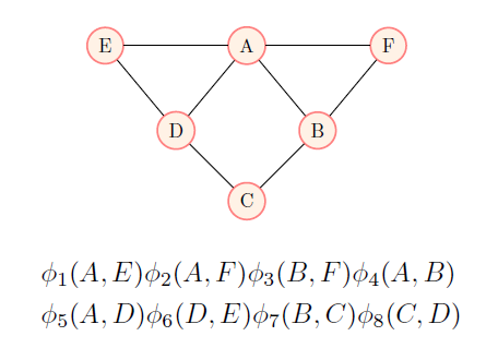
Now, because of the Hammersley–Clifford theorem, any probability distribution that has strictly positive density can be decomposed as a markov network \(G\) and potential functions \(\phi_{C \in \operatorname{cliques}(G)} : X_C \mapsto \mathbb{R}_{\geq 0}\) such that:
\[P(X=x) = \frac{\prod\limits_{C \in \operatorname{cliques}(G)} \phi_C (C = x_C)}{\sum\limits_{x'} \prod\limits_{C \in \operatorname{cliques}(G)} \phi_C (C = x_C)}\]Where \(x_C\) is \(x\) restricted to the random variables that are included in the clique \(C\).
Any distribution with strictly positive density can also be decomposed in exponential form as:
\[P(X=x) = \frac{ \exp \left( \sum\limits_{j=1}^{K} w_j f_j (x) \right) }{ \sum\limits_{x'} \exp \left( \sum\limits_{j=1}^{K} w_j f_j (x') \right) }\]Where the features \(f_j\) can be binary i.e. \(f_j(x) \in \{0,1 \}\) and \(exp(a) = e^a\).
In the most direct translation, there is one feature corresponding to each possible state of each clique. This representation is exponential in the size of the cliques.
However, we are free to specify a much smaller number of features (e.g., logical functions of the state of the clique) at the cost of lower representation domain i.e. we can fix \(K\) to a much lower number. This allows for a more compact representation than the potential-function form.
A distribution \(P\) is a log linear model over a Markov network \(G\) if it is associated with:
- A set of features \(\{ f_1(D_1) , ... , f_m(D_m) \}\) where each \(D_i\) is a clique of \(G\) and \(f\) takes value 1 for some values \(y \in Val(D)\) i.e. a condition. Note: we can have several features over the same clique.
- A set of weights \(w_1,...,w_m\) such that:
Where \(x \mid_{D_j}\) is the vector \(x\) restricted to the variables present in \(D_j\).