Markov Logic Networks

23 Oct 2019 Logic Learning Query answering Statistical relational Markov

Markov Logic Networks (Richardson & Domingos, 2006), a.k.a. MLN, is a representation and query answering framework that combines probability and first-order logic.

Some of the interesting things about this framework:

• It does not impose language restrictions other than finiteness of domain (constants).
• It is in essence a language to specify Markov networks.
• Handles uncertainty and contradictory knowledge.
• It works well in practical cases: collective classification, link prediction and social network modeling for instance.
• It learns weights on formulas in order to answer queries in the unit interval \([0,1]\) by considering the notion of possible worlds.

Markov networks

A markov network is an undirected graph \(G=(V,E)\) where \(V\) is a set of random variables and there is an edge \((X_i,X_j) \in E\) iff random variables \(X_j\) and \(X_i\) depend on each other. Meaning, any variable is conditionally independent from all others given its neightbors.

Any distribution with strictly positive density can be decomposed in exponential form (given the independence condition above) as:

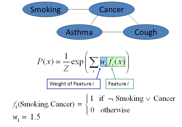
\[P(X=x) = \frac{ \exp \left( \sum\limits_{j=1}^{K} w_j f_j (x) \right) }{ \sum\limits_{x'} \exp \left( \sum\limits_{j=1}^{K} w_j f_j (x') \right) }\]

In the most direct translation, there is one feature corresponding to each possible state of each clique. However, we are free to specify a much smaller number of features, as a log-linear model (at the cost of precision):

\[P(X=x) = \frac{ \exp \left( \sum\limits_{j=1}^{m} w_j f_j (x \mid_{D_j}) \right) }{ \sum\limits_{x'} \exp \left( \sum\limits_{j=1}^{m} w_j f_j (x' \mid_{D_j}) \right) }\]

Where:

• Each \(D_i\) is a clique of \(G\) and \(f\) takes value 1 for some values \(y \in Val(D)\) i.e. a condition.
• \(x \mid_{D_j}\) is the vector \(x\) restricted to the variables present in \(D_j\).

Example:

Features can be learned from data, for example by greedily constructing conjunctions of atomic features (Della Pietra et al., 1997).

Network weights can be found efficiently using standard gradient-based or quasi-Newton optimization methods, because the log-likelihood is a concave function of the weights (Nocedal & Wright, 1999).

Logic and knowledge bases

Information can be represented by first-order knowledge bases, a set of closed formulas/sentences. Formulas are constructed as usual in first-order logic with a vocabulary consisting of predicate, function, variables and (finite) constant symbols.

A term is a constant, variable or function applied to other terms. An atom is a predicate applied to terms. A formula is a construct of atoms using the symbols \(\{\neg , \land , \lor , \forall , \exists , \Rightarrow \}\). A ground term/atom/formula does not contain any variables. A closed formula has no free (unquantified) variables.

A possible world assigns a truth value to each possible ground atom. A formula is satisfiable iff there exists at least one world in which it is true. A KB entails a formula \(F\) is every world that satisfies all sentences of KB, also satisfies \(F\).

Every KB in first-order logic can be converted to conjunctive normal form easily, while preserving satisfiability. Horn clauses, are clauses containing at most one positive literal.

We assume our KB is a set of Horn clauses.

Markov logic networks

In a MLN, formulas in the KB have an assigned weight. They are not seen as hard constraints, but rather as targets. The higher the weight a formulas has, the greater the difference in log probability (i.e. score) between a world that satisfies the formula and one that does not, other things being equal.

In simple terms, MLNs are an instantiation of Markov networks where the nodes (representing random variables) are ground atoms while edges represent that there is a formula where two ground atoms are present.

Formally, given \(L = \{ (F_1 , w_1) , (F_2 , w_2) , ... \}\) a set of pairs where \(F_i\) is a formula and \(w_i \in \mathbb{R}\) its weight, and \(C\) a finite set of constants, a markov logic network \(M_{L,C}=(V,E,D)\) is a markov network where:

• \(V\) contains one binary node for each atom appearing in any \(F_i\) w.r.t. \(C\).
• \((A_1,A_2) \in E\) iff there is a formula \(F_i\) such that \(A_1\) and \(A_2\) appear in it.
• \(D\) the set of features, contains one feature for each possible grounding of each formula \(F_i\) in \(L\).

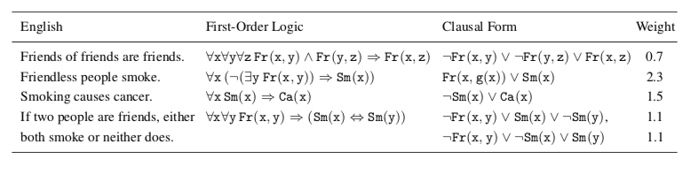
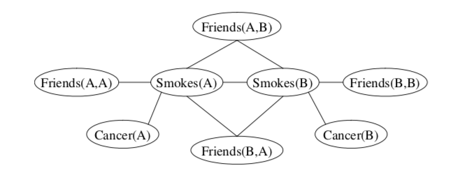
Example of a grounded MLN using the KB above with set of constants \(C=\{A,B\}\):

A possible world \(x\), is a mapping from each grounded atom in the MLN to \(\{0,1\}\) representing whether that predicate is true or false. The probability distribution over possible worlds \(x\) specified by the ground Markov network \(M_{L,C}\) is given by:

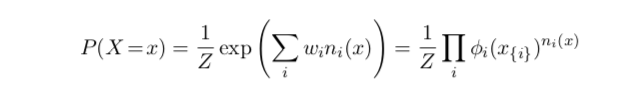
Where \(n_i(x)\) is the number of true groundings of \(F_i\) in \(x\), \(x_{\{i\}}\) is the state (truth values) of the atoms appearing in \(F_i\), and \(\phi_i(x_{\{i\}}) = e^{w_i}\) .

In order to restrict the graph to be finite, MLNs assume that:

1. Constants are given and finite.
2. For each function appearing in \(L\), the value of that function applied to every possible tuple of arguments is an element of \(C\).

MLNs preserve entailment in the following sense:

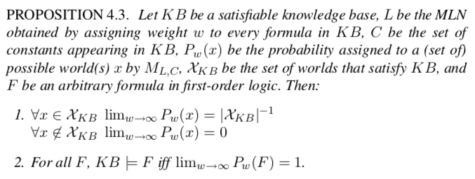
In other words, in the limit of all equal infinite weights, the MLN represents a uniform distribution over the worlds that satisfy the KB, and all entailment queries can be answered by computing the probability of the query formula and checking whether it is 1.

However, an MLN can produce useful results even when it contains contradictions.

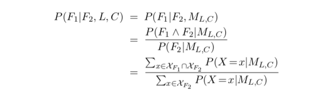
MLNs can answer arbitrary queries of the form “What is the probability that formula \(F_1\) holds given that formula \(F_2\) does?”:

They give an efficient implementation of inference by grounding the minimal subset of the network required for answering the query and running a Gibbs sampler over this subnetwork, with initial states found by MaxWalkSat.

Given a database, MLN weights can in principle be learned using standard methods, as follows. If the ith formula has \(n_i(x)\) true groundings in the data \(x\), then the derivative of the log-likelihood with respect to its weight is:

Where the sum is over all possible databases \(x'\).

Counting the number of true groundings of a formula in a database is intractable. But more efficient alternatives are presented in the paper. Weights are learned by optimizing a pseudo-likelihood measure using the L-BFGS algorithm, and clauses are learned using the CLAUDIEN system.

References

1. Richardson, M., & Domingos, P. (2006). Markov logic networks. Machine Learning, 62(1-2), 107–136.
   
2. Della Pietra, S., Della Pietra, V., & Lafferty, J. (1997). Inducing features of random fields. IEEE Transactions on Pattern Analysis and Machine Intelligence, 19(4), 380–393.
   
3. Nocedal, J., & Wright, S. J. (1999). Numerical optimization, P. Glynn and SM Robinson, eds. Springer.